class: center, middle, inverse, title-slide # Probabilistic<br> Forecast<br> Reconciliation ## Properties, Evaluation <br> and Score Optimisation ### Anastasios Panagiotelis ### September 23, 2020 --- class:center # Joint work with Puwasala Gamakumara <img src="img/puwac.jpg" width="100"/> -- George Athanasopoulos  -- Rob Hyndman  --- class: inverse, center, middle # Motivation --- # Hierarchical Time Series - Predictions of multiple variables needed. -- - Variables follow linear constraints. -- - Forecast store level sales and aggregates. <div id="htmlwidget-68d8889c5e5d2aa217df" style="width:100%;height:300px;" class="widgetframe html-widget"></div> <script type="application/json" data-for="htmlwidget-68d8889c5e5d2aa217df">{"x":{"url":"ProbReco_files/figure-html//widgets/widget_unnamed-chunk-1.html","options":{"xdomain":"*","allowfullscreen":false,"lazyload":false}},"evals":[],"jsHooks":[]}</script> --- # Electricity Example - Total daily electricity in Australian NEM -- - Renewable - Non-renewable -- - Renewable can be broken down -- - Solar - Wind - etc. -- - Solar can be broken down into -- - Solar rooftop - Solar utility -- - Data sourced from [Open NEM](opennem.org.au). --- # Electricity Data [<span style="color:white">(link)</span>](https://anastasiospanagiotelis.shinyapps.io/ProbRecoApp) <iframe src = 'https://anastasiospanagiotelis.shinyapps.io/ProbRecoApp' height=520 width=780 overflow-y='scroll' overflow-x='hidden'></iframe> --- # Main takeaways - Data have different characteristics regarding -- - Trends - Seasonality - Spikes - Signal to noise ratio -- - Hard to come up with a single multivariate model. -- - Even harder to do so while accounting for constraints. --- # Why multivariate? - Electricity cannot be economically stored at large scale (yet). -- - Day ahead load forecasting crucial input to dispatch and operational decisions. -- - Increased use of renewables result in uncertainty in supply. -- - Decisions of generators, market regulators may depend on total generation but also on generation from individual sources. -- - Avoid non-aligned decisions. --- # Why probabilistic? - Prices are heavily right skewed. -- - Prices in NSW reached $14700 on January 4th,2020. - This compares to $30-$40 on a normal day. -- - Price peaks coincide with the use of fuels with higher marginal cost. -- - Another important consideration is grid reliability. -- - Tails are important! --- class: middle, center, inverse # What is reconciliation? --- # Traditional approaches - Single level approaches -- - Bottom Up (Schwarzkopf, Tersine, and Morris, 1988). -- - Top Down (Gross and Sohl, 1990). -- - Middle Out -- - Top down do not exploit information at bottom levels. -- - Bottom up can suffer from the noisiness of bottom level series. -- - These approaches do not work for more general constraints. --- # Reconciliation .pull-left[ - Forecast every variable, stack in an `\(n\)`-vector `\(\hat{\mathbf{y}}\)`. - Call these .emphcol[base] forecasts. - Forecasts not .emphcol[coherent]. - Forecasts need to be .emphcol[reconciled] via a mapping `\(\tilde{\mathbf{y}}=\psi(\hat{\mathbf{y}})\)`. ] -- .pull-right[] --- # Some math Linear reconciliation generally takes the form `$$\tilde{\mathbf{b}}=\left(\mathbf{d}+\mathbf{G}\hat{\mathbf{y}}\right)$$` where -- - `\(\mathbf{G}\)` is an `\(m\times n\)` matrix of reconciliation weights - `\(\mathbf{d}\)` is `\(m\times 1\)` translation vector -- The full hierarchy is `\(\tilde{\mathbf{y}}=\mathbf{S}\tilde{\mathbf{b}}\)` where `\(\mathbf{S}\)` is an `\(n\times m\)` matrix that encodes constraints. --- # The summing matrix .pull-left[ <div id="htmlwidget-a47bc3a01ab31d4297ff" style="width:100%;height:300px;" class="widgetframe html-widget"></div> <script type="application/json" data-for="htmlwidget-a47bc3a01ab31d4297ff">{"x":{"url":"ProbReco_files/figure-html//widgets/widget_unnamed-chunk-2.html","options":{"xdomain":"*","allowfullscreen":false,"lazyload":false}},"evals":[],"jsHooks":[]}</script> ] --- # The summing matrix .pull-left[ <div id="htmlwidget-9183c4a5bd5411783334" style="width:100%;height:300px;" class="widgetframe html-widget"></div> <script type="application/json" data-for="htmlwidget-9183c4a5bd5411783334">{"x":{"url":"ProbReco_files/figure-html//widgets/widget_unnamed-chunk-3.html","options":{"xdomain":"*","allowfullscreen":false,"lazyload":false}},"evals":[],"jsHooks":[]}</script> ] .pull-right[ `\(\mathbf{S}=\begin{pmatrix}1&1&1&1\\1&1&0&0\\0&0&1&1\\1&0&0&0\\0&1&0&0\\0&0&1&0\\0&0&0&1\\\end{pmatrix}\)` ] --- # Specific reconciliation methods - OLS: `\(\tilde{\mathbf{y}}=\mathbf{S}\left(\mathbf{S}'\mathbf{S}\right)^{-1}\mathbf{S}'\hat{\mathbf{y}}\)` - Hyndman, Ahmed, Athanasopoulos, and Shang (2011) -- - WLS: `\(\tilde{\mathbf{y}}=\mathbf{S}\left(\mathbf{S}'\mathbf{W}\mathbf{S}\right)^{-1}\mathbf{S}'\mathbf{W}\hat{\mathbf{y}}\)` - Athanasopoulos, Hyndman, Kourentzes, and Petropoulos (2017) -- - MinT: `\(\tilde{\mathbf{y}}=\mathbf{S}\left(\mathbf{S}'\mathbf{\Sigma}^{-1}\mathbf{S}\right)^{-1}\mathbf{S}'\mathbf{\Sigma}^{-1}\hat{\mathbf{y}}\)` - Wickramasuriya, Athanasopoulos, and Hyndman (2019) --- class: inverse, middle center # Probabilistic forecasts --- # Existing approaches - Stack quantiles of each series in a vector and reconcile - Shang and Hyndman (2017) for prediction intervals. - Jeon, Panagiotelis, and Petropoulos (2019) (hereafter JPP) for a full distribution. -- - Reconcile mean otherwise bottom up - Ben Taieb, Taylor, and Hyndman (2020) (hereafter BTTH) --- # Formal Definition: Coherence - Let `\(\left(\mathbb{R}^m,\mathscr{F}_{\mathbb{R}^m},\mu\right)\)` be a probability triple - Let `\(s:\mathbb{R}^m\rightarrow\mathfrak{s}\)` where `\(s(.)\)` is premultiplication by `\(\mathbf{S}\)`. -- - A coherent probabilistic forecast can be characterised by a probability triple `\(\left(\mathfrak{s},\mathscr{F}_{\mathfrak{s}},\nu\right)\)` where `$$\nu(s(\mathcal{B}))=\mu(\mathcal{B})\quad\forall\mathcal{B}\in{\mathscr{F}_{\mathbb{R}^m}}$$` and `\(s(\mathcal{B})\)` is the image of `\(\mathcal{B}\)` under `\(s(.)\)`. 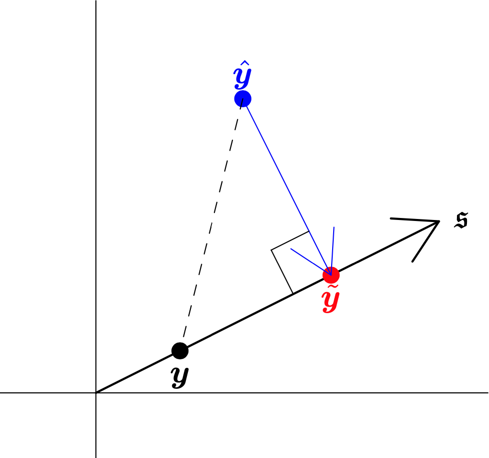--- # In a picture <img src="img/probforecoh_schematic.svg" width="80%" style="display: block; margin: auto;" /> --- # Formal Definition: Reconciliation Let `\(\left(\mathbb{R}^n,\mathscr{F}_{\mathbb{R}^n},\hat\nu\right)\)` be a probability triple corresponding to a base forecast. -- The reconcilied forecast is characterised by `$$\tilde\nu(\mathcal{A})=\hat\nu(\psi^{-1}(\mathcal{A}))\quad\forall\mathcal{A}\in\mathscr{F}_{\mathfrak{s}}$$` and `\(\psi^{-1}(\mathcal{A})\)` is the pre-image of `\(\mathcal{A}\)` under `\(\psi(.)\)`. --- # In a picture <img src="img/probforerec_schematic.svg" width="80%" style="display: block; margin: auto;" /> --- # In practice If `\(\hat{\mathbf{y}}^{[1]},\ldots,\hat{\mathbf{y}}^{[L]}\)` is a sample from some base probabilistic forecast, then `\(\tilde{\mathbf{y}}^{[1]},\ldots,\tilde{\mathbf{y}}^{[L]}\)` is a sample from the reconciled forecast where `$$\tilde{\mathbf{y}}^{[l]}=\psi(\hat{\mathbf{y}}^{[l]})\quad\forall l=1,\ldots,L$$` -- *Reconciling a sample from the base distribution gives a sample from the reconciled distribution.* -- Proof in paper. --- # In practice - If the base forecast is elliptical, then the reconcilied forecast will be elliptical. -- - If the base forecast is `\(\mathcal{N}(\hat{\boldsymbol{\mu}},\hat{\mathbf{\Sigma}})\)` -- - If reconciliation is linear `\(\psi(\hat{\mathbf{y}}):=\mathbf{S}\left(\mathbf{d}+\mathbf{G}\hat{\mathbf{y}}\right)\)` -- - The reconciled forecast is `\(\mathcal{N}\left(\mathbf{S}(\mathbf{d}+\mathbf{G}\hat{\boldsymbol{\mu}}),\mathbf{S}\mathbf{G}\hat{\mathbf{\Sigma}}\mathbf{G}'\mathbf{S}'\right)\)` --- # Perfect Reconciliation - Using the result on the previous slide we prove that for an arbitrary `\(\hat{\boldsymbol{\mu}}\)` and `\(\hat{\boldsymbol{\Sigma}}\)` there exists a `\(\mathbf{d}\)` and `\(\mathbf{G}\)` that recovers the true predictive distribution. -- - No matter how bad the base forecast is reconciliation can get you to the *truth*. -- - It is not feasible. -- - Will not always be a projection. --- class: inverse, center, middle # Score Optimisation --- #Scoring Rules - Propose reconciliation by optimising with respect to a *scoring rule* (Gneiting and Raftery, 2007). -- - A scoring rule `\(K(q,\boldsymbol{\omega})\)` takes a probabilistic forecast `\(q\)` and a realisation `\(\boldsymbol{\omega}\)` and returns a real number. -- - The rule is *proper* if `$$E_p\left[K(p,\omega)\right]\leq E_p\left[K(q,\omega)\right]$$` for all `\(p\neq q\)` where `\(\omega\sim p\)` --- # Multivariate scoring rules - Log score -- - Improper in context of reconciliation. - Result proven in paper. -- - Energy score -- - Multivariate generalisation of continuous ranked probability score. -- - Variogram score (Scheuerer and Hamill, 2015) --- # If `\(\mathbf{d}\)` and `\(\mathbf{G}\)` known Use training data `\(t=1,\ldots,T\)` to train models and make base forecasts. <div id="htmlwidget-e1509d434938c1920bbe" style="width:800px;height:200px;" class="DiagrammeR html-widget"></div> <script type="application/json" data-for="htmlwidget-e1509d434938c1920bbe">{"x":{"diagram":"\ngantt\ndateFormat YYYY-MM-DD\ntitle Forecast Setup\n\nTrain t=1 to t=T : obs_1, 2019-01-07, 4w\nForecast T+h :done, dec_1, after obs_1, 1d\n\n"},"evals":[],"jsHooks":[]}</script> -- Then reconcile. --- # Training `\(\mathbf{d}\)` and `\(\mathbf{G}\)` <div id="htmlwidget-19e339debde67d63624b" style="width:800px;height:400px;" class="DiagrammeR html-widget"></div> <script type="application/json" data-for="htmlwidget-19e339debde67d63624b">{"x":{"diagram":"\ngantt\ndateFormat YYYY-MM-DD\ntitle Forecast Setup\nsection Reco. Weights\n1st Training Window : obs_2, 2019-01-01, 4w\n1st Score :crit, dec_2, after obs_2, 1d\n2nd Training Window : obs_3, 2019-01-02, 4w\n2nd Score :crit, after obs_3, 1d\n3rd Training Window : obs_4, 2019-01-03, 4w\n3rd Score :crit, after obs_4, 1d\nRth Training Window : obs_6, 2019-01-06, 4w\nRth Score :crit, after obs_6, 1d\nsection Forecasting\nTrain t=R+1 to t=T+R : obs_1, 2019-01-07, 4w\nForecast T+R+h :done, dec_1, after obs_1, 1d\n"},"evals":[],"jsHooks":[]}</script> --- # In math Optimise `$$\mathcal{E}\left(\boldsymbol{\gamma}\right)=\sum\limits_{t=T}^{T+R-1} \textit{K}(\tilde{f}^{\boldsymbol{\gamma}}_{t+h|t},\mathbf{y}_{t+h})$$` -- where `\(\tilde{f}^{\boldsymbol{\gamma}}_{t+h|t}\)` is reconciled with respect to `\(\boldsymbol{\gamma}:=(\mathbf{d},vec(\mathbf{G}))\)` -- - Energy and variogram score approximated via Monte Carlo. --- # Energy Score `$$\mathcal{E}\left(\boldsymbol{\gamma}\right)\approx\sum\limits_{t=T}^{T+R-1}\left[\frac{1}{Q}\bigg(\sum\limits_{q=1}^{Q}||\tilde{\boldsymbol{y}}^{[q]}_{t+h|t}-\boldsymbol{y}_{t+h}||\right.\\-\left.\frac{1}{2}||\tilde{\boldsymbol{y}}_{t+h|t}^{[q]}-\tilde{\boldsymbol{y}}^{*[q]}_{t+h|t}||\bigg)\right]$$` -- `\(\tilde{\boldsymbol{y}}^{[q]}_{t+h|t}=\boldsymbol{S}\big(\boldsymbol{d}+\boldsymbol{G}{\hat{\boldsymbol{y}}}^{[q]}_{t+h|t}\big)\)`, `\(\tilde{\boldsymbol{y}}^{*[q]}_{t+h|t}=\boldsymbol{S}\big(\boldsymbol{d}+\boldsymbol{G}{\hat{\boldsymbol{y}}}^{*[q]}_{t+h|t}\big)\)` and `\({\hat{\boldsymbol{y}}}^{[q]}_{t+h|t},{\hat{\boldsymbol{y}}}^{*[q]}_{t+h|t}\overset{iid}{\sim} \hat{f}_{t+h|t}\)` for `\(q=1,\ldots,Q\)` --- #Stochastic Gradient Descent - When the objective function is only known up to approximation *Stochastic Gradient Descent* can be used for optimisation. -- - Requires an estimate of the gradient found by Automatic Differentiation. -- - The specific variant of SGD used is Adam (Kingma and Ba, 2014). -- - Implementation available in [ProbReco](https://cran.r-project.org/web/packages/ProbReco/index.html) package. --- class: inverse, center, middle # Simulation --- # Scenarios Simulate from 7-variable hierarchy with bottom levels given by ARIMA models -- - Stationary Gaussian -- - Stationary non-Gaussian -- - Non-stationary Gaussian -- - Non-stationary non-Gaussian --- # Base forecasts Obtain point forecasts from ARIMA or ETS models. To sample from base probabilistic forecasts add noise that is -- - Independent Gaussian noise -- - Multivariate Gaussian noise -- - Bootstraped residuals -- - Jointly bootstapped residuals --- # Residual Matrix `$$\begin{pmatrix}e_{\mathrm{Tot},1}&\cdots&e_{\mathrm{Tot},t}&\cdots&e_{\mathrm{Tot},T}\\ e_{A,1}&\cdots&e_{A,t}&\cdots&e_{A,T}\\ e_{B,1}&\cdots&e_{B,t}&\cdots&e_{B,T}\\ e_{AA,1}&\cdots&e_{AA,t}&\cdots&e_{AA,T}\\ e_{AB,1}&\cdots&e_{AB,t}&\cdots&e_{AB,T}\\ e_{BA,1}&\cdots&e_{BA,t}&\cdots&e_{BA,T}\\ e_{BB,1}&\cdots&e_{BB,t}&\cdots&e_{BB,T}\end{pmatrix}\\$$` --- # Independently Bootstapped `$$\begin{pmatrix}e_{\mathrm{Tot},1}&\cdots&\color{blue}{e_{\mathrm{Tot},t}}&\cdots&e_{\mathrm{Tot},T}\\ \color{blue}{e_{A,1}}&\cdots&e_{A,t}&\cdots&e_{A,T}\\ \color{blue}{e_{B,1}}&\cdots&e_{B,t}&\cdots&e_{B,T}\\ e_{AA,1}&\cdots&e_{AA,t}&\cdots&\color{blue}{e_{AA,T}}\\ \color{blue}{e_{AB,1}}&\cdots&e_{AB,t}&\cdots&e_{AB,T}\\ e_{BA,1}&\cdots&e_{BA,t}&\cdots&\color{blue}{e_{BA,T}}\\ e_{BB,1}&\cdots&\color{blue}{e_{BB,t}}&\cdots&e_{BB,T}\end{pmatrix}\\$$` --- # Jointly Bootstapped `$$\begin{pmatrix}e_{\mathrm{Tot},1}&\cdots&\color{blue}{e_{\mathrm{Tot},t}}&\cdots&e_{\mathrm{Tot},T}\\ e_{A,1}&\cdots&\color{blue}{e_{A,t}}&\cdots&e_{A,T}\\ e_{B,1}&\cdots&\color{blue}{e_{B,t}}&\cdots&e_{B,T}\\ e_{AA,1}&\cdots&\color{blue}{e_{AA,t}}&\cdots&e_{AA,T}\\ e_{AB,1}&\cdots&\color{blue}{e_{AB,t}}&\cdots&e_{AB,T}\\ e_{BA,1}&\cdots&\color{blue}{e_{BA,t}}&\cdots&e_{BA,T}\\ e_{BB,1}&\cdots&\color{blue}{e_{BB,t}}&\cdots&e_{BB,T}\end{pmatrix}$$` --- # Reconciliation methods - JPP: Reconcile quantiles. -- - BTTH: Reconcile mean, otherwise BU. -- - BU: Bottom up. -- - OLS: Orthogonal projection. -- - MinT: With shrinkage estimator. -- - ScoreOptE: Optimise w.r.t Energy Score. -- - ScoreOptV: Optimise w.r.t Variogram Score. --- # Simulation Results [<span style="color:white">(link)</span>](https://anastasiospanagiotelis.shinyapps.io/ProbRecoSim) <iframe src = 'https://anastasiospanagiotelis.shinyapps.io/ProbRecoSim/' height=520 width=780 overflow-y='scroll'></iframe> --- class: inverse, middle, center # Energy application --- # Base forecasts Use a feed-forward neural network with up to 28 lags of daily data. For probabilisitic forecasts: -- - Independent Gaussian noise -- - Multivariate Gaussian noise -- - Bootstraped residuals -- - Jointly bootstapped residuals -- Consider day-ahead forecasts. 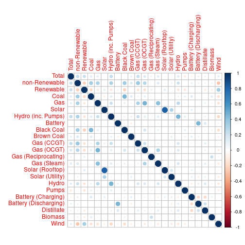--- # Model Fit [<span style="color:white">(link)</span>](https://anastasiospanagiotelis.shinyapps.io/ProbRecoApp) <iframe src = 'https://anastasiospanagiotelis.shinyapps.io/ProbRecoApp' height=520 width=780 overflow-y='scroll'></iframe> --- # Residual Dependence <img src="ProbReco_files/figure-html/unnamed-chunk-8-1.png" style="display: block; margin: auto;" /> --- # Reconciliation Results <img src="img/meanenergyscore.svg" height="560" style="display: block; margin: auto;" /> --- # Independent Gaussian <img src="img/nemenyi_ig.svg" height="560" style="display: block; margin: auto;" /> --- # Joint Bootstrap <img src="img/nemenyi_jb.svg" height="560" style="display: block; margin: auto;" /> --- # Main takeaway - Score optimisation dominates alternatives when base forecasts are badly mis-specified. -- - If base models are good then OLS dominates. -- - Existing approaches in the literature do not work well and are even dominated by base forecasts. -- - Possible bias-variance tradeoff at play. Future work may look at regularised approaches to score optimisation. --- # References .small[ Athanasopoulos, G. et al. (2017). "Forecasting with temporal hierarchies". In: _European Journal of Operational Research_ 262.1, pp. 60-74. Ben Taieb, S. et al. (2020). "Hierarchical Probabilistic Forecasting of Electricity Demand With Smart Meter Data". In: _Journal of the American Statistical Association_. in press. Gneiting, T. et al. (2007). "Strictly Proper Scoring Rules, Prediction, and Estimation". In: _Journal of the American Statistical Association_ 102.477, pp. 359-378. Gross, C. W. et al. (1990). "Disaggregation methods to expedite product line forecasting". In: _Journal of Forecasting_ 9.3, pp. 233-254. Hyndman, R. J. et al. (2011). "Optimal combination forecasts for hierarchical time series". In: _Computational Statistics and Data Analysis_ 55.9, pp. 2579-2589. Jeon, J. et al. (2019). "Probabilistic forecast reconciliation with applications to wind power and electric load". In: _European Journal of Operational Research_ 279.2, pp. 364-379. Kingma, D. P. et al. (2014). "Adam: A method for stochastic optimization". . http://arxiv.org/abs/1412.6980. Scheuerer, M. et al. (2015). "Variogram-Based Proper Scoring Rules for Probabilistic Forecasts of Multivariate Quantities". In: _Monthly Weather Review_ 143.4, pp. 1321-1334. Schwarzkopf, A. B. et al. (1988). "Top-down versus bottom-up forecasting strategies". In: _International Journal of Production Research_ 26 (11), pp. 1833-1843. Shang, H. L. et al. (2017). "Grouped Functional Time Series Forecasting: An Application to Age-Specific Mortality Rates". In: _Journal of Computational and Graphical Statistics_ 26.2, pp. 330-343. Wickramasuriya, S. L. et al. (2019). "Optimal Forecast Reconciliation for Hierarchical and Grouped Time Series Through Trace Minimization". In: _Journal of the American Statistical Association_ 114.526, pp. 804-819. ]